Determining Cardiac Axis

The cardiac axis refers to the general direction in which the heart depolarises.

Each wave of depolarisation begins at the Sinoatrial node, then spreads to the Atrioventricular node, before travelling to the Bundle of HIS and the Purkinje fibres to complete an electrical cardiac cycle.

When viewing the heart from the front, imagine a clock face. In the case of a normal cardiac conduction pathway, the wave of electrical activity travels from 11 o’clock to 5 o’clock.

 

A pathology that affects the conduction pathway of the heart will therefore affect the way the wave of depolarisation causes the heart to contract.

There are more than a couple of factors that influence cardiac axis:

Those of an anatomical persuasion:

• The heart’s anatomical position in the thoracic cavity (dextrocardia), or abnormal thoracic anatomy
• Abnormal diaphragm position (pregnancy and obesity, among others)

And those that are pathological, some examples of which are:

• Conduction abnormailities
• Prior myocardial infarction
• Pulmonary embolism
• Hypertrophy
• Ischaemia

With regards to the hexaxial reference system, the RAD and LAD denote Right and Left Axis Deviation, respectively.

Right Axis Deviation

• Depolarisation skewed rightward:1 o’clock to 7 o’clock
• Leads I and aVF deflection= negative (dominant S wave)
• Leads aVF and III= positive (dominant R wave)
• Usually cased by right ventricular hypertrophy
  • Increased mass of right ventricle. Associated with pulmonary conditions
• Can be a normal finding in very tall patients.

(It is important to note that some axis deviations from the norm are not uncommon In certain types of individual)

Left Axis Deviation

• Depolarisation skewed leftward
• Leads I and aVL= positive (dominant R wave)
• Leads II and aVF= negative (dominant S wave)
• Usually due to conduction abnormalities, as oppose to increased LV mass.

There are a number of ways (of varying accuracy) via which to calculate a cardiac axis using an ECG and the hexaxial reference system, pictured below.

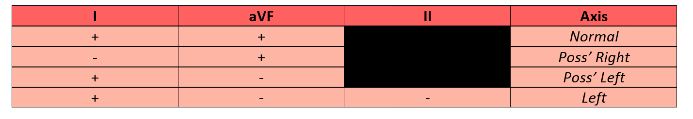
Method 1. The Quickest Way

It’s as simple as following this table:

Method 2. The Nearest 30°

• Identify the most isoelectric lead on the ECG and then on the hexaxial reference diagram
• Find the axis line that crosses this lead at 90°
• Determine the direction of the axis line by via the lead trace on the ECG.
  • If it is positive:
    • It travels towards the lead
  • If it is negative:
    • It travels away from the lead

Worked example:

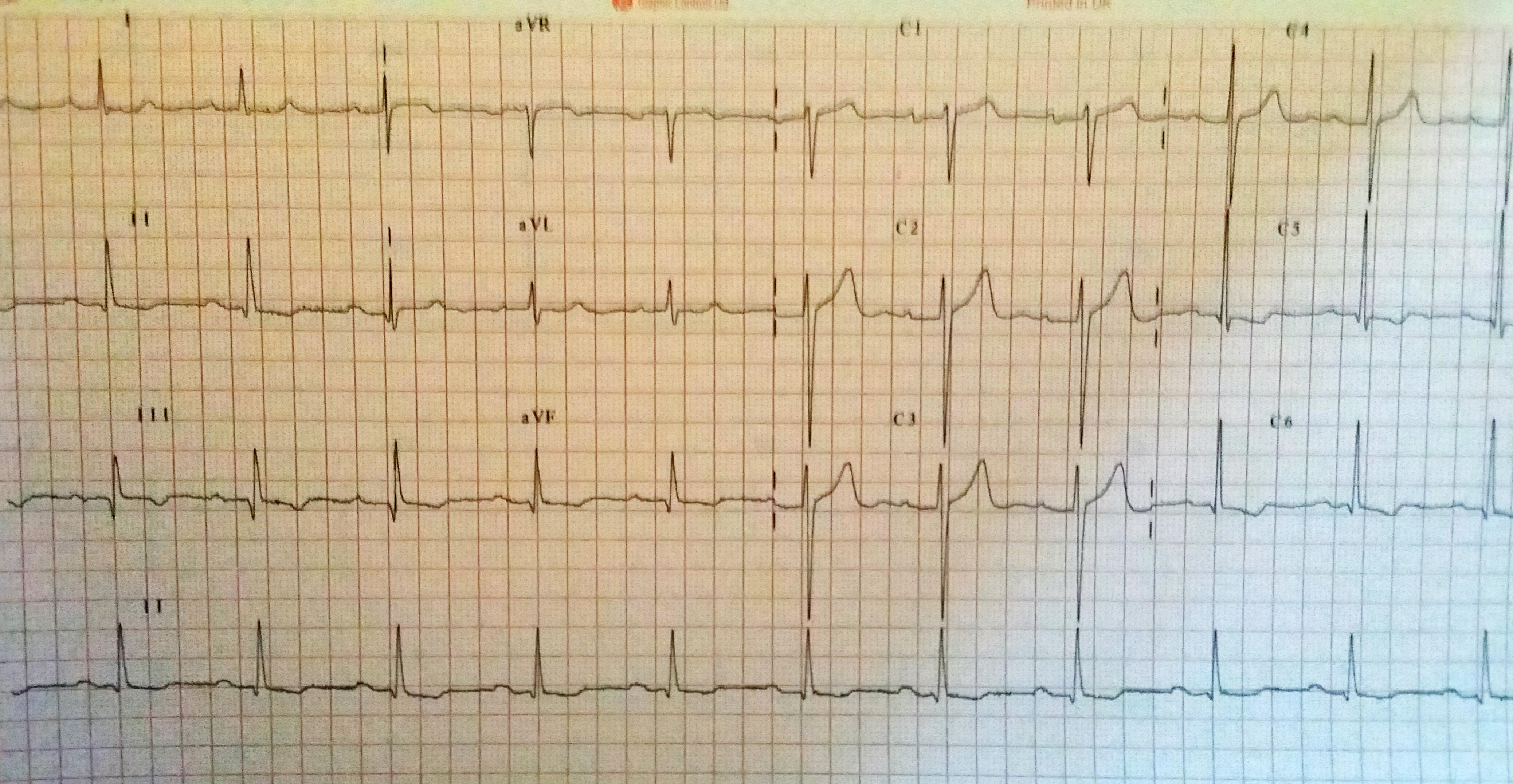
• Looking at the ECG pictured, we can see that aVL is the most isoelectric lead.
• On the diagram, lead II crosses it at 90°
• Lead II shows a positive deflection on the ECG, so on the diagram, we move towards the arrow and to +60°, ergo:
• This patient has a normal cardiac axis

Method 3. The Precise Calculation

This method isn’t commonly used, clinically, but it’s a method regardless. Plus, you never know if you’ll need it.

• Measure lead I’s overall height on the trace
  • R-S (mm)
• Measure lead aVF overall height on the trace
  • R-S (mm)
• Plug these numbers into the following diagram:

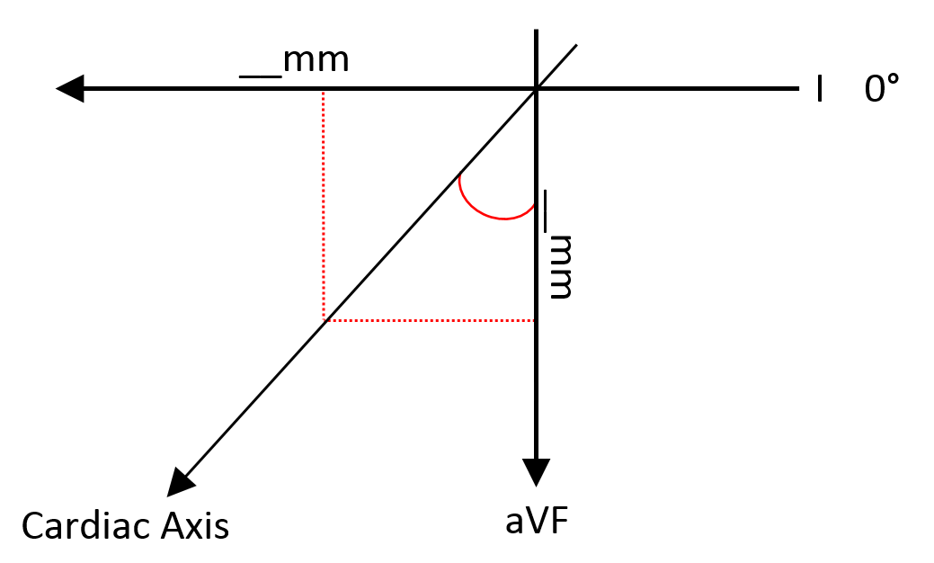
• Then this formula:

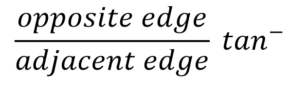
• This provides the cardiac axis
  • If both leads I and aVF are positive, this figure stands
  • If not, add 90° to the calculated figure

Worked example:

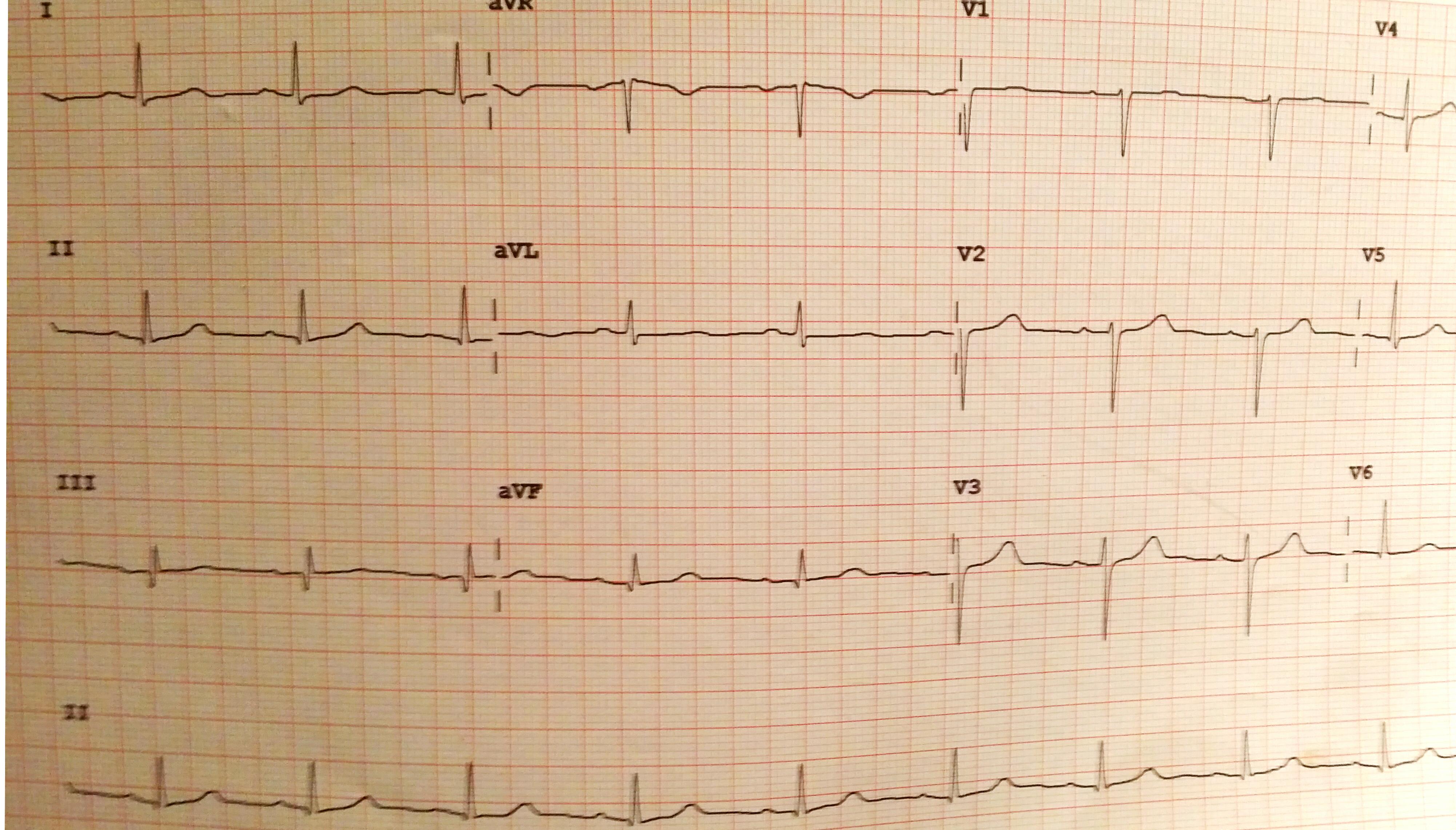
• Lead I R-S: 7-2= 5mm
• Lead aVF R-S: 5-0= 5mm
• tan^–(5/5) = 45
• Refer back to the diagram. 45° falls within the normal parameters, so:
• This patient has a normal cardiac axis

Use the first two methods to test the third one!